Google Sheets has developed into a crucial tool for information organization and analysis in the modern world, which is increasingly data-driven. When it comes to data lookup and retrieval, VLOOKUP’s ability to revolutionize the process is just one of many superpowers it possesses.
This Google Sheets VLOOKUP tutorial is here to walk you through everything you need to know about making this tool work its magic in the real world, regardless of whether you are just starting out or consider yourself to be an old hand.
Understanding VLOOKUP:
Before we jump into the nitty-gritty, let’s break down what VLOOKUP is and why it’s a rock star in the data world. VLOOKUP, or “Vertical Lookup” for the uninitiated, is a function that lets you hunt for a value in a specific range or table and fetch a related value from the same row. It’s like having a data detective at your service, saving you hours of manual data hunting and headaches.
Imagine being able to effortlessly locate that vital piece of information amidst a sea of data, like finding a needle in a haystack. VLOOKUP is your trusty compass in the data wilderness, guiding you to the exact data point you need, whether you’re dealing with pricing details, inventory lists, or customer records. It’s your secret weapon for making informed decisions and unraveling insights hidden within your datasets. So, let’s embark on this VLOOKUP journey and unlock the full potential of your data prowess.
Why VLOOKUP in Google Sheets Matters
VLOOKUP is more than a fancy formula; it’s a data hero. Here’s why it’s the MVP in your Google Sheets toolkit:
- Efficiency: VLOOKUP automates the grunt work of finding and grabbing data, leaving you with more time to interpret and act on your findings.
- Accuracy: Say goodbye to human errors in data retrieval; VLOOKUP ensures your data is spot on.
- Scale: From small tasks to colossal projects, VLOOKUP handles data of all sizes with ease.
Now that we’re singing VLOOKUP’s praises, let’s roll up our sleeves and learn how to use it like a pro.
Getting Started with VLOOKUP in Google Sheets
To kick off your VLOOKUP adventure, follow these simple steps:
Step 1: Data Prep 101
Before you let VLOOKUP work its magic, tidy up your data. Here’s a quick checklist:
- Your data should be neatly organized in columns.
- Each column needs a unique heading.
- The search key (the thing you’re looking for) should live in the leftmost column of your data.
Step 2: Writing the VLOOKUP Formula
Now comes the fun part—crafting your VLOOKUP formula. Here’s a sneak peek:=(=VLOOKUP(search_key, range, col_index, [range_lookup])
- search_key: The value you’re hunting for.
- range: The table where you’ll go searching.
- col_index: The column number from which to grab your data.
- [range_lookup]: An optional setting that tells VLOOKUP whether to find an exact match (FALSE) or a close one (TRUE).
Step 3: Let VLOOKUP Do Its Thing
Once your formula is cooked up, hit Enter, and watch the magic happen. Let’s put theory into practice:
Imagine you have a list of products and their prices. You want to find the price of a product called “Widget.” With VLOOKUP, it’s a breeze.
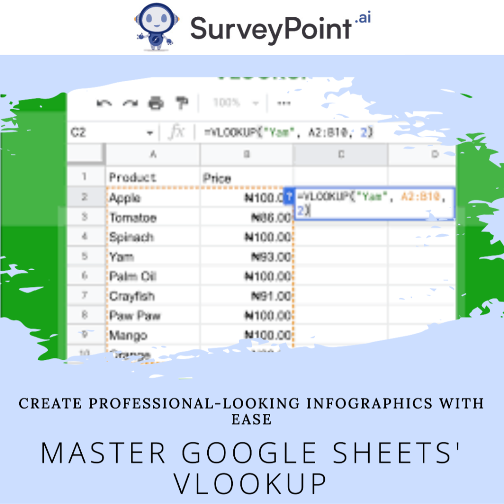
VLOOKUP in Action: A Real-World Example
Your data looks like this:
- Product Name (Column A)
- Price (Column B)
You’re on a quest to find the price of the elusive “Widget.” Your VLOOKUP formula goes like this:=VLOOKUP(“Widget”, A2:B10, 2, FALSE)
Here’s the breakdown:
- “Widget”: The product name you’re hunting for
- A2:B10: Where your data hangs out
- 2: The magic number (column index) where the price lives
- False: The setting for an exact match
Voilà! Google Sheets serves up the price of your “Widget” on a silver platter.
Pitfalls to Dodge
While VLOOKUP is your trusty sidekick, be aware of these common gotchas:
- Data Type Drama: Check to see that the data type you are searching for and the data associated with your search key are the same. If your search key is text, your data should also be text.
- It is Important to Use Dollar Signs: Whenever you copy your VLOOKUP formula to other cells, make sure to use dollar signs ($) to lock cell references. When you apply the formula to multiple rows, this helps to ensure that the results are accurate.
- The Drama of Missing Data In the event that your search key does not locate a match, VLOOKUP will throw an error. You can handle this in a dignified manner by using the IFERROR function to show a custom message instead of the standard one.
- Approximate Match Awareness: Exercise caution when working with the range_lookup setting, which is completely optional. Your data must be sorted in ascending order for it to be considered a TRUE match (an approximate match). For precision, stick with FALSE.
Conclusion
In a nutshell, mastering VLOOKUP in Google Sheets will boost your data analysis skills to superhero levels. With these steps and a mindful eye on common blunders, you’ll conquer data challenges with finesse and accuracy.
Remember, practice is the key to mastery. Dive into your own Google Sheets projects, experiment, and see VLOOKUP’s magic in action. Armed with this knowledge, you’re well on your way to becoming a data wizard.
